@WangEtAl2021

Cite

Wang, Chien-Yao, Alexey Bochkovskiy, and Hong-Yuan Mark Liao. “Scaled-YOLOv4: Scaling Cross Stage Partial Network.” arXiv, February 21, 2021. http://arxiv.org/abs/2011.08036.

Synth

Contribution::

Md

Author:: Wang, Chien-Yao

Author:: Bochkovskiy, Alexey

Author:: Liao, Hong-Yuan Mark

Title:: Scaled-YOLOv4: Scaling Cross Stage Partial Network
Year:: 2021
Citekey:: @WangEtAl2021

Tags:: Computer Science - Computer Vision and Pattern Recognition, 🏷️, Computer Science - Machine Learning, 📙
itemType:: preprint

LINK

Wang et al_2021_Scaled-YOLOv4.pdf.

Abstract

abstract:: We show that the YOLOv4 object detection neural network based on the CSP approach, scales both up and down and is applicable to small and large networks while maintaining optimal speed and accuracy. We propose a network scaling approach that modifies not only the depth, width, resolution, but also structure of the network. YOLOv4-large model achieves state-of-the-art results: 55.5% AP (73.4% AP50) for the MS COCO dataset at a speed of ~16 FPS on Tesla V100, while with the test time augmentation, YOLOv4-large achieves 56.0% AP (73.3 AP50). To the best of our knowledge, this is currently the highest accuracy on the COCO dataset among any published work. The YOLOv4-tiny model achieves 22.0% AP (42.0% AP50) at a speed of 443 FPS on RTX 2080Ti, while by using TensorRT, batch size = 4 and FP16-precision the YOLOv4-tiny achieves 1774 FPS.

---

Annotations

Highlight

We propose a network scaling approach that modifies not only the depth, width, resolution, but also structure of the network. (Go to Paper)

1. Introduction

Highlight

In order to design an effective object detector, model scaling technique is very important, because it can make object detector achieve high accuracy and real-time inference on various types of devices. (Go to Paper)

Highlight

he most common model scaling technique is to change the depth (number of layers in a neural network) and width (number of filters in a layer) of the backbone, and then train neural networks suitable for different devices. (Go to Paper)

Image

Image

Highlight

In [2], Cai et al. try to develop techniques that can be applied to various device network architectures with only training once. They use techniques such as decoupling training and search and knowledge distillation to decouple and train several sub-nets, so that the entire network and sub-nets are capable of processing target tasks. (Go to Paper)

Comment:

Cai 등은 다양한 장치 네트워크 구조에 단 한 번의 훈련으로 적용할 수 있는 기술을 개발하려고 시도합니다. 그들은 훈련과 탐색을 분리하고 지식 증류와 같은 기술을 사용하여 여러 서브넷을 분리하고 훈련함으로써 전체 네트워크와 서브넷이 모두 대상 작업을 처리할 수 있도록 합니다. 이러한 접근 방식은 네트워크의 효율성과 유연성을 향상시키려는 노력의 일환입니다. 여기서 ‘훈련과 탐색의 분리’는 모델을 훈련시키는 과정과 최적의 구조를 탐색하는 과정을 별도로 진행함을 의미합니다. ‘지식 증류’는 큰 모델이나 네트워크로부터 학습된 정보를 보다 작은 모델이나 네트워크로 전달하는 기법을 말합니다. 이를 통해, 작은 모델이나 서브넷도 전체 네트워크와 유사한 성능을 낼 수 있도록 합니다. 이런 방식으로, 한 번의 훈련으로 다양한 장치와 네트워크 구조에 쉽게 적용할 수 있는 모델을 개발할 수 있는 것이 목표입니다.

Highlight

Tan et al. [34] proposed using network architecture search (NAS) technique to perform compound scaling width, depth, and resolution on EfficientNet-B0. They use this initial network to search for the best convolutional neural network (CNN) architecture for a given amount of computation and set it as EfficientNet-B1, and then use linear scale-up technique to obtain EfficientNet-B2 to EfficientNet-B7. (Go to Paper)

Comment:

Tan 등은 EfficientNet-B0에 복합 스케일링을 수행하기 위해 네트워크 아키텍처 탐색(NAS) 기술을 사용하는 것을 제안했습니다. 복합 스케일링은 너비, 깊이, 해상도를 조정하는 것을 의미합니다. 그들은 이 초기 네트워크를 사용하여 주어진 계산량에 대해 최적의 합성곱 신경망(CNN) 아키텍처를 탐색하고, 이를 EfficientNet-B1로 설정합니다. 그 후, 선형 스케일 업 기술을 사용하여 EfficientNet-B2부터 EfficientNet-B7까지 얻습니다. 이 과정에서 NAS는 다양한 네트워크 구조를 자동으로 탐색하고 평가하여, 주어진 자원(예: 계산량) 내에서 가장 효율적인 모델 구조를 찾아냅니다. 이러한 방법을 통해, EfficientNet-B0를 기반으로 하여 다양한 크기의 네트워크를 효율적으로 설계할 수 있으며, 각기 다른 요구 사항(예: 더 높은 정확도, 더 적은 계산 비용)에 맞추어 최적화된 모델을 생성할 수 있습니다. EfficientNet-B1은 이러한 탐색 과정을 통해 결정된 아키텍처를 바탕으로 하며, 이후 모델들은 EfficientNet-B1의 구조를 유지하면서 너비, 깊이, 해상도를 선형적으로 확장함으로써 성능을 개선합니다. 이렇게 함으로써, 각기 다른 성능 수준을 요구하는 다양한 응용 프로그램에 적합한 모델 시리즈를 제공할 수 있습니다.

Highlight

Radosavovic et al. [27] summarized and added constraints from the vast parameter search space AnyNet, and then designed RegNet to find optimal depth, bottleneck ratio, and width increase rate of a CNN. In addition, there are NAS and model scaling methods specifically proposed for object detection [6, 35]. (Go to Paper)

Comment:

Radosavovic 등은 매우 넓은 매개변수 탐색 공간인 AnyNet에서 요약하고 제약 조건을 추가한 후, CNN의 최적 깊이, 병목 비율, 그리고 너비 증가율을 찾기 위해 RegNet을 설계했습니다. 또한, 객체 탐지를 위해 특별히 제안된 NAS(네트워크 아키텍처 탐색) 및 모델 스케일링 방법도 있습니다. 여기서 AnyNet은 다양한 아키텍처 구성을 탐색할 수 있는 네트워크 설계 공간을 의미합니다. Radosavovic 등은 이 넓은 공간 내에서 효율적인 탐색을 가능하게 하기 위해 추가적인 제약 조건을 도입하고, 이를 바탕으로 RegNet을 설계했습니다. RegNet은 깊이(depth), 병목 비율(bottleneck ratio), 그리고 너비 증가율(width increase rate) 같은 주요 매개변수들의 최적 조합을 찾아 CNN의 성능을 극대화합니다. 객체 탐지와 같은 특정 응용 프로그램을 위해서는, NAS와 모델 스케일링 방법이 특별히 제안되었습니다. 이는 객체 탐지에 최적화된 아키텍처와 모델 크기를 결정하기 위해, 특별한 요구 사항과 제약 조건을 고려하는 과정을 포함합니다. 이러한 방법들은 객체 탐지의 정확도와 효율성을 향상시키기 위해 개발되었으며, 다양한 계산 자원과 환경에서 뛰어난 성능을 발휘할 수 있는 모델을 생성하는 데 중점을 둡니다.

Highlight

Through analysis of state-of-the-art object detectors [1, 3, 6, 26, 35, 40, 44], we found that CSPDarknet53, which is the backbone of YOLOv4 [1], matches almost all optimal architecture features obtained by network architecture search technique [27]. (Go to Paper)

Highlight

In the proposed scaled-YOLOv4, we discussed the upper and lower bounds of linear scaling up/down models, and respectively analyzed the issues that need to be paid attention to in model scaling for small models and large models. Thus, we are able to systematically develop YOLOv4-large and YOLOv4-tiny models. (Go to Paper)

Highlight

We summarize the contributions of this paper : (1) design a powerful model scaling method for small model, which can systematically balance the computation cost and memory bandwidth of a light CNN; (2) design a simple yet effective strategy for scaling a large object detector; (3) analyze the relations among all model scaling factors and then perform model scaling based on most advantageous group partitions; (4) experiments have confirmed that the FPN structure is inherently a once-for-all structure; and (5) we make use of the above methods to develop YOLOv4-tiny and YOLOv4-large. (Go to Paper)

Comment:

*이 논문의 기여도를 요약하면 다음과 같습니다:

1. 소형 모델을 위한 강력한 모델 스케일링 방법을 설계하여, 경량 CNN의 계산 비용과 메모리 대역폭을 체계적으로 균형잡을 수 있습니다.
2. 큰 객체 탐지기를 스케일링하기 위한 단순하지만 효과적인 전략을 설계합니다.
3. 모든 모델 스케일링 요소들 사이의 관계를 분석한 후, 가장 유리한 그룹 분할에 기반하여 모델 스케일링을 수행합니다.
4. 실험을 통해 FPN(Feature Pyramid Network) 구조가 본질적으로 일회용(once-for-all) 구조임을 확인했습니다.
5. 위의 방법들을 활용하여 YOLOv4-tiny와 YOLOv4-large를 개발했습니다. 설명: 1번 기여도는 소형 모델에 적합한 모델 스케일링 방법을 개발함으로써, 자원이 제한된 환경에서도 효율적인 성능을 낼 수 있는 CNN을 설계할 수 있음을 의미합니다. 이는 경량화된 모델이 필요한 임베디드 시스템이나 모바일 디바이스에서 특히 유용합니다. 2번 기여도는 대형 객체 탐지 모델의 성능을 개선하기 위한 전략을 제공함으로써, 더 큰 정확도와 효율성을 달성할 수 있게 합니다. 3번에서는 모델 스케일링 과정에서 고려해야 할 다양한 요소들 간의 상호작용을 이해하고, 이를 바탕으로 최적의 구성을 찾는 방법을 제시합니다. 4번 기여도는 FPN 구조가 다양한 크기와 형태의 모델에 유연하게 적용될 수 있음을 보여줍니다. 이는 객체 탐지 분야에서 중요한 발견으로, 다양한 응용 프로그램에 적용 가능한 범용적인 구조를 제시합니다. 마지막으로, 5번 기여도는 위에서 논의한 모든 기술적 진보를 통합하여, 실제로 YOLOv4의 두 가지 변형 모델을 개발했음을 강조합니다. 이를 통해 더 넓은 범위의 응용 분야에서 YOLOv4의 활용 가능성을 확장시킵니다.*

2. Related work

2.1. Real-time object detection

Highlight

Object detectors is mainly divided into one-stage object detectors [28, 29, 30, 21, 18, 24] and two-stage object detectors [10, 9, 31]. The output of one-stage object detector can be obtained after only one CNN operation. As for twostage object detector, it usually feeds the high score region proposals obtained from the first-stage CNN to the secondstage CNN for final prediction. The inference time of onestage object detectors and two-stage object detectors can be expressed as Tone = T1st and Ttwo = T1st + mT2nd , where m is the number of region proposals whose confidence score is higher than a threshold. Today’s popular real-time object detectors are almost one-stage object detectors. Onestage object detectors mainly have two kinds: anchor-based [30, 18] and anchor-free [7, 13, 14, 36]. Among all anchorfree approaches, CenterNet [46] is very popular because it does not require complicated post-processing, such as NonMaximum Suppression (NMS). At present, the more accurate real-time one-stage object detectors are anchor-based EfficientDet [35], YOLOv4 [1], and PP-YOLO [22]. In this paper, we developed our model scaling methods based on YOLOv4 [1]. (Go to Paper)

Comment:

1단계 객체 탐지기는 한 번의 CNN 연산으로 객체의 위치와 종류를 직접 예측하는 방식으로, 빠른 처리 속도 때문에 실시간 시스템에 적합합니다. 반면, 2단계 객체 탐지기는 먼저 객체가 있을 법한 영역을 제안하고, 이후 이 영역들을 대상으로 더 정밀한 객체 검출을 수행하여 정확도를 높입니다. 앵커 기반 방식은 미리 정의된 앵커 박스를 사용하여 객체를 탐지하는 반면, 앵커 프리 방식은 앵커 박스 없이 객체의 중심점 등을 직접 예측하는 방식을 말합니다. 본 논문에서는 YOLOv4, 실시간 처리가 가능하면서도 높은 정확도를 제공하는 앵커 기반 1단계 객체 탐지기를 활용하여 새로운 모델 스케일링 방법을 개발하였습니다.

2.2. Model scaling

Highlight

Traditional model scaling method is to change the depth of a model, that is to add more convolutional layers. (Go to Paper)

Comment:

전통적 모델 스케일링은 주로 모델의 깊이를 늘리는 방식으로, 더 많은 합성곱 계층을 추가하여 모델을 깊게 만듦으로써 성능을 향상시키려는 전략입니다. VGGNet은 이러한 접근 방식의 대표적 예로, 다양한 버전에서 계층의 수를 조절하여 성능을 달리합니다. ResNet은 이를 한 단계 더 발전시켜, 매우 깊은 네트워크를 구축하여 성능을 대폭 향상시켰습니다.

Highlight

The subsequent methods generally follow the same methodology for model scaling. (Go to Paper)

Highlight

[43] thought about the width of the network, and they changed the number of kernel of convolutional layer to realize scaling. They therefore design wide ResNet (WRN) , while maintaining the same accuracy. Although WRN has higher amount of parameters than ResNet, the inference speed is much faster. (Go to Paper)

Comment:

이후 네트워크의 너비에 주목한 연구들도 등장했으며, WRN은 너비를 증가시킴으로써 더 빠른 추론 속도와 높은 성능을 달성했습니다.

Highlight

The subsequent DenseNet [12] and ResNeXt [41] also designed a compound scaling version that puts depth and width into consideration. (Go to Paper)

Comment:

복합 스케일링을 도입한 DenseNet과 ResNeXt는 깊이와 너비를 동시에 고려하여 더욱 향상된 모델을 제안했습니다.

Highlight

As for image pyramid inference, it is a common way to perform augmentation at run time. It takes an input image and makes a variety of different resolution scaling, and then input these distinct pyramid combinations into a trained CNN. Finally, the network will integrate the multiple sets of outputs as its ultimate outcome. Redmon et al. [30] use the above concept to execute input image size scaling. They use higher input image resolution to perform fine-tune on a trained Darknet53, and the purpose of executing this step is to get higher accuracy. (Go to Paper)

Comment:

이미지 피라미드 추론은 다양한 해상도의 이미지를 네트워크에 입력하여 더 높은 정확도를 얻기 위한 방법으로, 입력 이미지의 크기를 조절하여 성능을 미세 조정하는 전략입니다. 이러한 다양한 스케일링 방법은 모델의 성능을 최적화하고, 특히 고해상도 이미지 처리에 있어 더 높은 정확도를 달성하기 위한 노력의 일환입니다.

Highlight

In recent years, network architecture search (NAS) related research has been developed vigorously, and NASFPN [8] has searched for the combination path of feature pyramid. We can think of NAS-FPN as a model scaling technique which is mainly executed at the stage level. (Go to Paper)

Comment:

최근 NAS 연구는 네트워크 구조를 최적화하여 더 효율적인 모델을 설계하기 위한 방법으로 주목받고 있습니다. NAS-FPN은 특징 피라미드의 다양한 조합을 탐색하여 객체 탐지의 정확도를 높이는 데 중점을 둡니다.

Highlight

As for EfficientNet [34], it uses compound scaling search based on depth, width, and input size. The main design concept of EfficientDet [35] is to disassemble the modules with different functions of object detector, and then perform scaling on the image size, width,BiFPN layers, andclass layer. (Go to Paper)

Comment:

EfficientNet과 EfficientDet은 각각 깊이, 너비, 입력 크기 등 다양한 차원에서 모델을 스케일링하여 성능을 극대화하는 복합 스케일링 전략을 채택합니다. 이들은 객체 탐지기의 성능을 개선하기 위해 모델의 다양한 요소를 조정합니다.

Highlight

Another design that uses NAS concept is SpineNet [6], which is mainly aimed at the overall architecture of fish-shaped object detector for network architecture search. This design concept can ultimately produce a scalepermuted structure. Another network with NAS design is RegNet [27], which mainly fixes the number of stage and input resolution, and integrates all parameters such as depth, width, bottleneck ratio and group width of each stage into depth, initial width, slope, quantize, bottleneck ratio, and group width. Finally, they use these six parameters to perform compound model scaling search. (Go to Paper)

Comment:

SpineNet과 RegNet은 NAS를 이용하여 전체 네트워크 구조를 최적화하며, 특히 RegNet은 깊이, 너비, 병목 비율 등을 종합적으로 고려한 복합 스케일링 탐색을 수행합니다.

Highlight

The above methods are all great work, but few of them analyze the relation between different parameters. (Go to Paper)

Comment:

이러한 접근 방식은 모델의 성능을 효율적으로 향상시키지만, 다양한 매개변수 간의 상호 작용을 충분히 분석하는 데에는 한계가 있습니다.

Highlight

In this paper, we will try to find a method for synergistic compound scaling based on the design requirements of object detection. (Go to Paper)

Comment:

본 논문은 이러한 문제를 해결하기 위해 객체 탐지의 요구 사항에 맞춰 서로 보완적인 방식으로 모델을 스케일링하는 새로운 방법을 모색합니다. 이는 객체 탐지 분야에서 더욱 정교하고 효율적인 모델 설계로 이어질 수 있습니다.

3. Principles of model scaling

Highlight

After performing model scaling for the proposed object detector, the next step is to deal with the quantitative factors that will change, including the number of parameters with qualitative factors. These factors include model inference time, average precision, etc. The qualitative factors will have different gain effects depending on the equipment or database used. (Go to Paper)

3.1. General principle of model scaling

Highlight

When designing the efficient model scaling methods, our main principle is that when the scale is up/down, the lower/higher the quantitative cost we want to increase/decrease, the better. In this section, we will show and analyze various general CNN models, and try to understand their quantitative costs when facing changes in (1) image size, (2) number of layers, and (3) number of channels. The CNNs we chose are ResNet, ResNext, and Darknet. (Go to Paper)

Highlight

For the k-layer CNNs with b base layer channels, the computations of ResNet layer is k∗[conv(1 × 1, b/4) → conv(3 × 3, b/4) → conv(1 × 1, b)], and that of ResNext layer is k∗[conv(1 × 1, b/2) → gconv(3 × 3/32, b/2) → conv(1 × 1, b)]. As for the Darknet layer, the amount of computation is k∗[conv(1 × 1, b/2) → conv(3 × 3, b)]. (Go to Paper)

Highlight

Let the scaling factors that can be used to adjust the image size, the number of layers, and the number of channels be α, β, and γ, respectively. (Go to Paper)

Image

Image

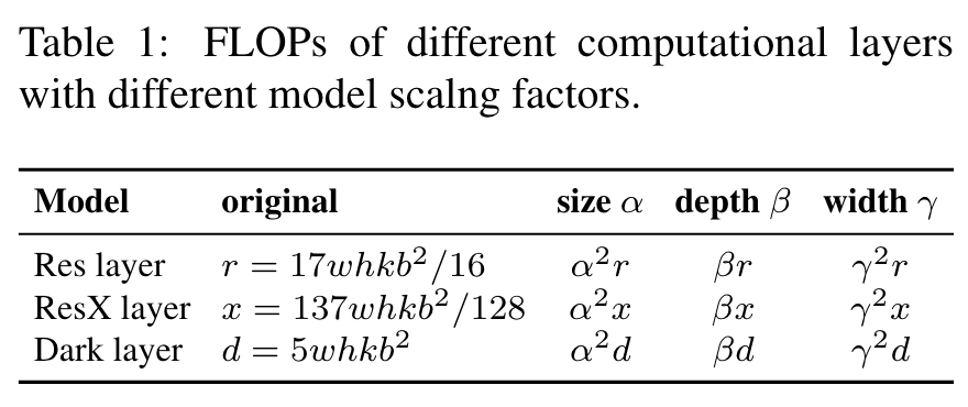
Highlight

the scaling size, depth, and width cause increase in the computation cost. They respectively show square, linear, and square increase. (Go to Paper)

Highlight

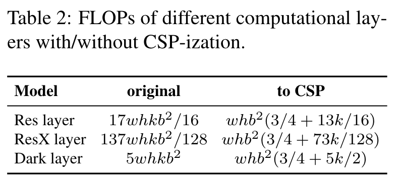
The CSPNet [37] proposed by Wang et al. can be applied to various CNN architectures, while reducing the amount of parameters and computations. In addition, it also improves accuracy and reduces inference time. We apply it to ResNet, ResNeXt, and Darknet and observe the changes in the amount of computations, as shown in Table 2. (Go to Paper)

Highlight

From the figures shown in Table 2, we observe that after converting the above CNNs to CSPNet, the new architecture can effectively reduce the amount of computations (FLOPs) on ResNet, ResNeXt, and Darknet by 23.5%, 46.7%, and 50.0%, respectively. Therefore, we use CSP-ized models as the best model for performing model scaling. (Go to Paper)

Image

Image

3.2. Scaling Tiny Models for Low-End Devices

Highlight

For low-end devices, the inference speed of a designed model is not only affected by the amount of computation and model size, but more importantly, the limitation of peripheral hardware resources must be considered. Therefore, when performing tiny model scaling, we must also consider factors such as memory bandwidth, memory access cost (MACs), and DRAM traffic. In order to take into account the above factors, our design must comply with the following principles: (Go to Paper)

Make the order of computations less than O(whkb2):

Highlight

Lightweight models are different from large models in that their parameter utilization efficiency must be higher in order to achieve the required accuracy with a small amount of computations. (Go to Paper)

Highlight

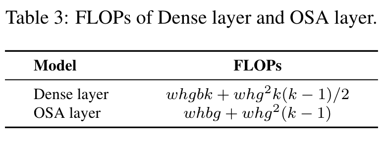
In Table 3, we analyze the network with efficient parameter utilization, such as the computation load of DenseNet and OSANet [15], where g means growth rate. (Go to Paper)

Image

Image

Highlight

For general CNNs, the relationship among g, b, and k listed in Table 3 is k << g < b. Therefore, the order of computation complexity of DenseNet is O(whgbk), and that of OSANet is O(max(whbg, whkg2)). The order of computation complexity of the above two is less than O(whkb2) of the ResNet series. Therefore, we design our tiny model with the help of OSANet, which has a smaller computation complexity. (Go to Paper)

Minimize/balance size of feature map:

Highlight

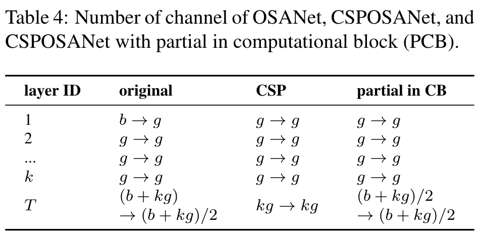
In order to get the best trade-off in terms of computing speed, we propose a new concept, which is to perform gradient truncation between computational block of the CSPOSANet. (Go to Paper)

Highlight

If we apply the original CSPNet design to the DenseNet or ResNet architectures, because the jth layer output of these two architectures is the integration of the 1st to (j − 1)th layer outputs, we must treat the entire computational block as a whole. (Go to Paper)

Highlight

Because the computational block of OSANet belongs to the PlainNet architecture, making CSPNet from any layer of a computational block can achieve the effect of gradient truncation. We use this feature to re-plan the b channels of the base layer and the kg channels generated by computational block, and split them into two paths with equal channel numbers, as shown in Table 4. (Go to Paper)

Image

Image

Highlight

When the number of channel is b + kg, if one wants to split these channels into two paths, the best partition is to divide it into two equal parts, i.e. (b + kg)/2. When we actually consider the bandwidth τ of the hardware, if software optimization is not considered, the best value is ceil((b + kg)/2τ ) × τ . The CSPOSANet we designed can dynamically adjust the channel allocation. (Go to Paper)

Maintain the same number of channels after convolution:

Highlight

For evaluating the computation cost of low-end device, we must also consider power consumption, and the biggest factor affecting power consumption is memory access cost (MAC). Usually the MAC calculation method for a convolution operation is as follows: M AC = hw(Cin + Cout) + KCinCout (1) where h, w, Cin, Cout, and K represent, respectively, the height and width of feature map, the channel number of input and output, and the kernel size of convolutional filter. By calculating geometric inequalities, we can derive the smallest MAC when Cin = Cout [23]. (Go to Paper)

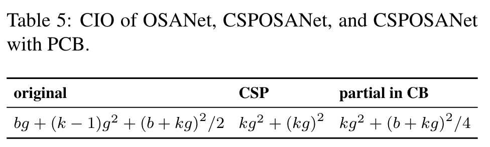
Minimize Convolutional Input/Output (CIO):

Highlight

CIO [4] is an indicator that can measure the status of DRAM IO. Table 5 lists the CIO of OSA, CSP, and our designed CSPOSANet. (Go to Paper)

Image

Image

Highlight

When kg > b/2, the proposed CSPOSANet can obtain the best CIO. (Go to Paper)

3.3. Scaling Large Models for High-End GPUs

Highlight

Since we hope to improve the accuracy and maintain the real-time inference speed after scaling up the CNN model, we must find the best combination among the many scaling factors of object detector when performing compound scaling. Usually, we can adjust the scaling factors of an object detector’s input, backbone, and neck. (Go to Paper)

Image

Image

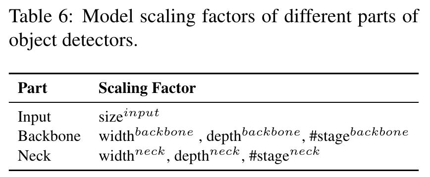
Highlight

The biggest difference between image classification and object detection is that the former only needs to identify the category of the largest component in an image, while the latter needs to predict the position and size of each object in an image. (Go to Paper)

Highlight

In one-stage object detector, the feature vector corresponding to each location is used to predict the category and size of an object at that location. The ability to better predict the size of an object basically depends on the receptive field of the feature vector. In the CNN architecture, the thing that is most directly related to receptive field is the stage, and the feature pyramid network (FPN) architecture tells us that higher stages are more suitable for predicting large objects. (Go to Paper)

Comment:

이 부분에서 저자들은 이미지 분류와 객체 탐지의 핵심 차이점을 강조하고 있습니다. 이미지 분류는 이미지에서 주요 객체의 분류만을 식별하는 반면, 객체 탐지는 더 복잡한 과제로, 이미지 내 모든 객체의 위치와 크기까지 파악해야 합니다. 이는 1단계 객체 탐지기에서 중요한데, 여기서는 위치별로 할당된 특징 벡터를 통해 객체의 카테고리와 크기 정보를 예측합니다. 이 예측 능력은 특징 벡터가 가진 수용 필드의 크기에 기반하는데, 이는 CNN 아키텍처의 다양한 ‘스테이지’에 의해 결정됩니다. FPN 아키텍처는 이를 활용하여 다양한 크기의 객체를 효과적으로 탐지할 수 있는 구조를 제공합니다. 논문의 표 7에서는 수용 필드의 크기와 다른 매개변수들과의 관계를 시각적으로 보여주며, 이는 모델이 객체의 크기를 정확하게 인식하는 데 필수적인 요소임을 나타냅니다.

Image

Image

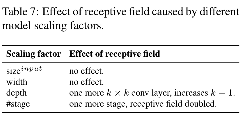
Highlight

From Table 7, it is apparent that width scaling can be independently operated. (Go to Paper)

Highlight

When the input image size is increased, if one wants to have a better prediction effect for large objects, he/she must increase the depth or number of stages of the network. (Go to Paper)

Highlight

Among the parameters listed in Table 7, the compound of {sizeinput,stage} turns out with the best impact. Therefore, when performing scaling up, we first perform compound scaling on sizeinput,stage, and then according to real-time requirements, we further perform scaling on depth and width respectively. (Go to Paper)

4. Scaled-YOLOv4

4.1. CSP-ized YOLOv4

Highlight

In this sub-section, we re-design YOLOv4 to YOLOv4-CSP to get the best speed/accuracy trade-off. (Go to Paper)

Backbone:

Highlight

In the design of CSPDarknet53, the computation of down-sampling convolution for cross-stage process is not included in a residual block. Therefore, we can deduce that the amount of computation of each CSPDarknet stage is whb2(9/4+3/4+5k/2). From the formula deduced above, we know that CSPDarknet stage will have a better computational advantage over Darknet stage only when k > 1 is satisfied. The number of residual layer owned by each stage in CSPDarknet53 is 1-2-8-8-4 respectively. In order to get a better speed/accuracy trade-off, we convert the first CSP stage into original Darknet residual layer. (Go to Paper)

Comment:

CSPDarknet53 아키텍처에서는 다운-샘플링을 위한 컨볼루션 연산이 잔차 블록의 일부로 계산되지 않는 특별한 설계를 적용합니다. 이로 인해 각 스테이지의 계산량은 너비(wh), 기본 채널 수(b), 그리고 컨볼루션 레이어 수(k)를 변수로 하는 특정 수식에 의해 결정됩니다. 이 수식에 따르면, 컨볼루션 레이어 수(k)가 1보다 클 경우에만 CSPDarknet53이 기존 Darknet 아키텍처에 비해 계산상의 이점을 가질 것으로 예측됩니다.CSPDarknet53는 다양한 단계에서 서로 다른 수의 잔차 레이어를 가지며, 이는 각 스테이지의 계산 복잡성에 영향을 미칩니다. 이러한 구성을 통해, 개발자들은 속도와 정확도 사이의 최적의 균형을 찾으려고 합니다. 특히 첫 번째 CSP 스테이지를 원래의 Darknet 잔차 레이어 구조로 변경함으로써, 모델이 빠른 속도에서도 높은 정확도를 유지할 수 있도록 최적화합니다. 이러한 조정은 실제 사용 환경에서의 성능을 향상시킬 수 있는 중요한 디자인 결정입니다.

Image

Image

Neck:

Highlight

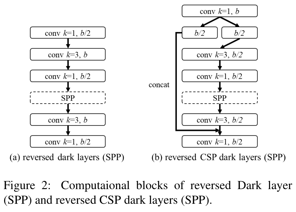
In order to effectively reduce the amount of computation, we CSP-ize the PAN [20] architecture in YOLOv4. The computation list of a PAN architecture is illustrated in Figure 2(a). It mainly integrates the features coming from different feature pyramids, and then passes through two sets of reversed Darknet residual layer without shortcut connections. After CSP-ization, the architecture of the new computation list is shown in Figure 2(b). This new update effectively cuts down 40% of computation. (Go to Paper)

SPP:

Highlight

The SPP module was originally inserted in the middle position of the first computation list group of the neck. Therefore, we also inserted SPP module in the middle position of the first computation list group of the CSPPAN. (Go to Paper)

4.2. YOLOv4-tiny

Image

Image

Highlight

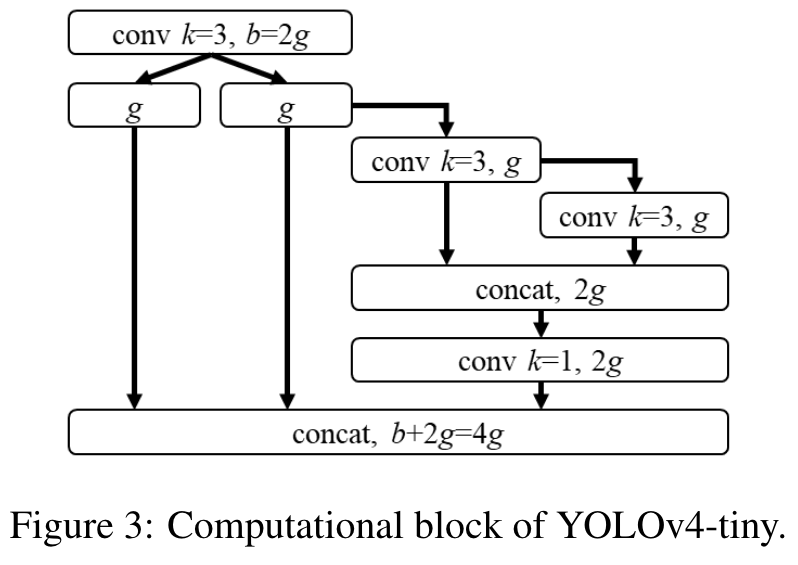
We will use the CSPOSANet with PCB architecture to form the backbone of YOLOv4. We set g = b/2 as the growth rate and make it grow to b/2 + kg = 2b at the end. Through calculation, we deduced k = 3, and its architecture is shown in Figure 3. As for the number of channels of each stage and the part of neck, we follow the design of YOLOv3-tiny. (Go to Paper)

4.3. YOLOv4-large

Highlight

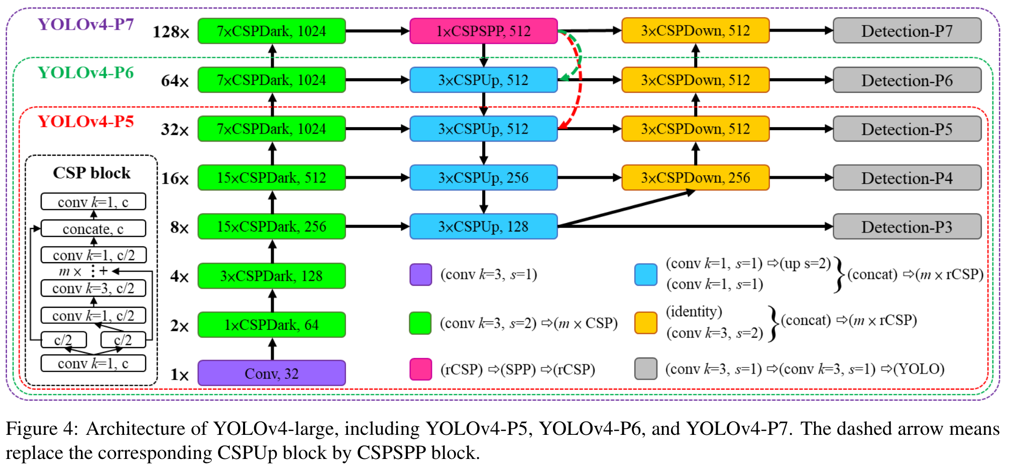
YOLOv4-large is designed for cloud GPU, the main purpose is to achieve high accuracy for object detection. We designed a fully CSP-ized model YOLOv4-P5 and scaling it up to YOLOv4-P6 and YOLOv4-P7. (Go to Paper)

Highlight

Figure 4 shows the structure of YOLOv4-P5, YOLOv4P6, and YOLOv4-P7. We designed to perform compound scaling on sizeinput,stage. We set the depth scale of each stage to 2dsi , and ds to [1, 3, 15, 15, 7, 7, 7]. Finally, we further use inference time as constraint to perform additional width scaling. Our experiments show that YOLOv4P6 can reach real-time performance at 30 FPS video when the width scaling factor is equal to 1. For YOLOv4-P7, it can reach real-time performance at 16 FPS video when the width scaling factor is equal to 1.25. (Go to Paper)

Comment:

이 부분에서 저자들은 YOLOv4의 세 가지 버전, 즉 YOLOv4-P5, YOLOv4-P6, YOLOv4-P7의 설계 구조와 스케일링 전략을 소개하고 있습니다. 복합 스케일링은 모델의 입력 크기와 스테이지 수에 동시에 적용되며, 각 스테이지의 깊이는 지수적으로 조정됩니다. 깊이 스케일링 인자 ���dsi는 모델의 각 스테이지마다 다르게 설정되어, 모델의 계층적 구조에 따라 다양한 계산 복잡성을 가지게 합니다.추가적으로, 추론 시간을 고려하여 모델의 너비 스케일링을 조정함으로써, 실제 비디오 처리에서의 실시간 성능을 달성하기 위한 최적의 조건을 찾고자 합니다. YOLOv4-P6와 YOLOv4-P7 모두에서, 너비 스케일링 인자를 조절함으로써 각각 30 FPS와 16 FPS에서의 실시간 비디오 처리 성능을 달성할 수 있음을 실험을 통해 확인했습니다. 이는 고성능 객체 탐지 모델을 실시간 애플리케이션에 적용할 수 있는 가능성을 보여줍니다.

5. Experiments

Highlight

We use MSCOCO 2017 object detection dataset to verify the proposed scaled-YOLOv4. We do not use ImageNet pre-trained models, and all scaled-YOLOv4 models are trained from scratch and the adopted tool is SGD optimizer. The time used for training YOLOv4-tiny is 600 epochs, and that used for training YOLOv4-CSP is 300 epochs. As for YOLOv4-large, we execute 300 epochs first and then followed by using stronger data augmentation method to train 150 epochs. As for the Lagrangian multiplier of hyper-parameters, such as anchors of learning rate, the degree of different data augmentation methods, we use k-means and genetic algorithms to determine. All details related to hyper-parameters are elaborated in Appendix. (Go to Paper)

Image

Image

Image

Image

Image

Image

Image

Image

5.1. Ablation study on CSP-ized model

Highlight

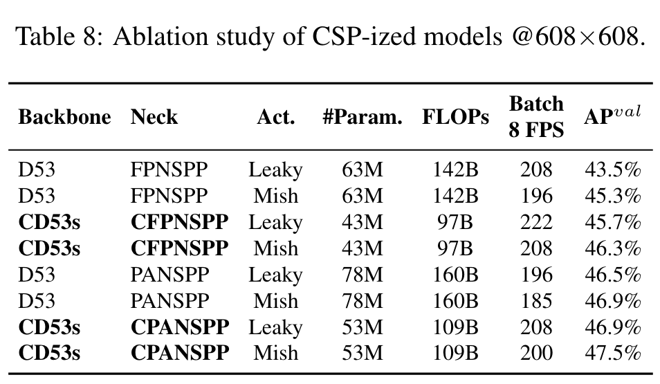
we will CSP-ize different models and analyze the impact of CSP-ization on the amount of parameters, computations, throughput, and average precision. (Go to Paper)

Highlight

We use Darknet53 (D53) as backbone and choose FPN with SPP (FPNSPP) and PAN with SPP (PANSPP) as necks to design ablation studies. (Go to Paper)

Highlight

We use LeakyReLU (Leaky) and Mish activation function respectively to compare the amount of used parameters, computations, and throughput. Experiments are all conducted on COCO minval dataset and the resulting APs are shown in the last column of Table 8. (Go to Paper)

Highlight

From the data listed in Table 8, it can be seen that the CSP-ized models have greatly reduced the amount of parameters and computations by 32%, and brought improvements in both Batch 8 throughput and AP. (Go to Paper)

Highlight

If one wants to maintain the same frame rate, he/she can add more layers or more advanced activation functions to the models after CSP-ization. (Go to Paper)

Highlight

we can see that both CD53s-CFPNSPP-Mish, and CD53sCPANSPP-Leaky have the same batch 8 throughput with D53-FPNSPP-Leaky, but they respectively have 1% and 1.6% AP improvement with lower computing resources. (Go to Paper)

Highlight

From the above improvement figures, we can see the huge advantages brought by model CSP-ization. Therefore, we decided to use CD53s-CPANSPP-Mish, which results in the highest AP in Table 8 as the backbone of YOLOv4-CSP. (Go to Paper)

5.2. Ablation study on YOLOv4-tiny

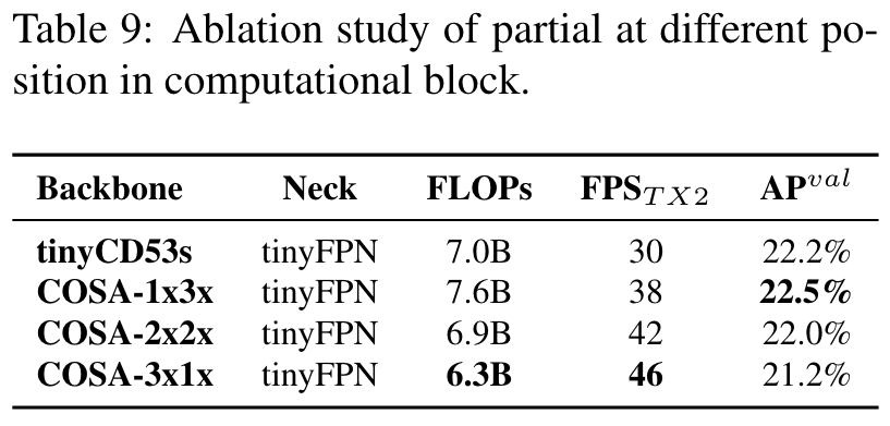
Highlight

In this sub-section, we design an experiment to show how flexible can be if one uses CSPNet with partial functions in computational blocks. We also compare with CSPDarknet53, in which we perform linear scaling down on width and depth. The results are shown in Table 9. (Go to Paper)

Image

Image

Highlight

we can see that the designed PCB technique can make the model more flexible, because such a design can be adjusted according to actual needs. (Go to Paper)

Highlight

we also confirmed that linear scaling down does have its limitation. It is apparent that when under limited operating conditions, the residual addition of tinyCD53s becomes the bottleneck of inference speed, because its frame rate is much lower than the COSA architecture with the same amount of computations. (Go to Paper)

Comment:

위의 결과들로부터, 우리는 선형 축소가 그 한계를 가지고 있음을 또한 확인했습니다. 제한된 운영 조건 하에서, tinyCD53s의 잔여 추가가 추론 속도의 병목이 되는 것이 분명하며, 이는 같은 계산량을 가진 COSA 아키텍처보다 프레임 속도가 훨씬 낮기 때문입니다.

Highlight

we also see that the proposed COSA can get a higher AP. Therefore, we finally chose COSA-2x2x which received the best speed/accuracy trade-off in our experiment as the YOLOv4-tiny architecture. (Go to Paper)

5.3. Ablation study on YOLOv4-large

Highlight

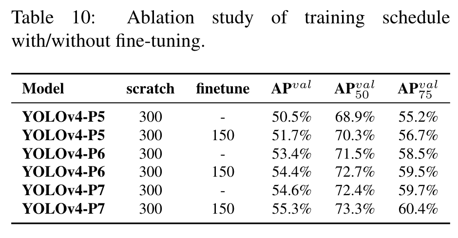
In Table 10 we show the AP obtained by YOLOv4 models in training from scratch and fine-tune stages. (Go to Paper)

5.4. Scaled-YOLOv4 for object detection

Highlight

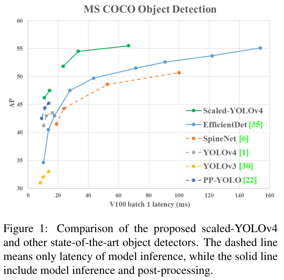
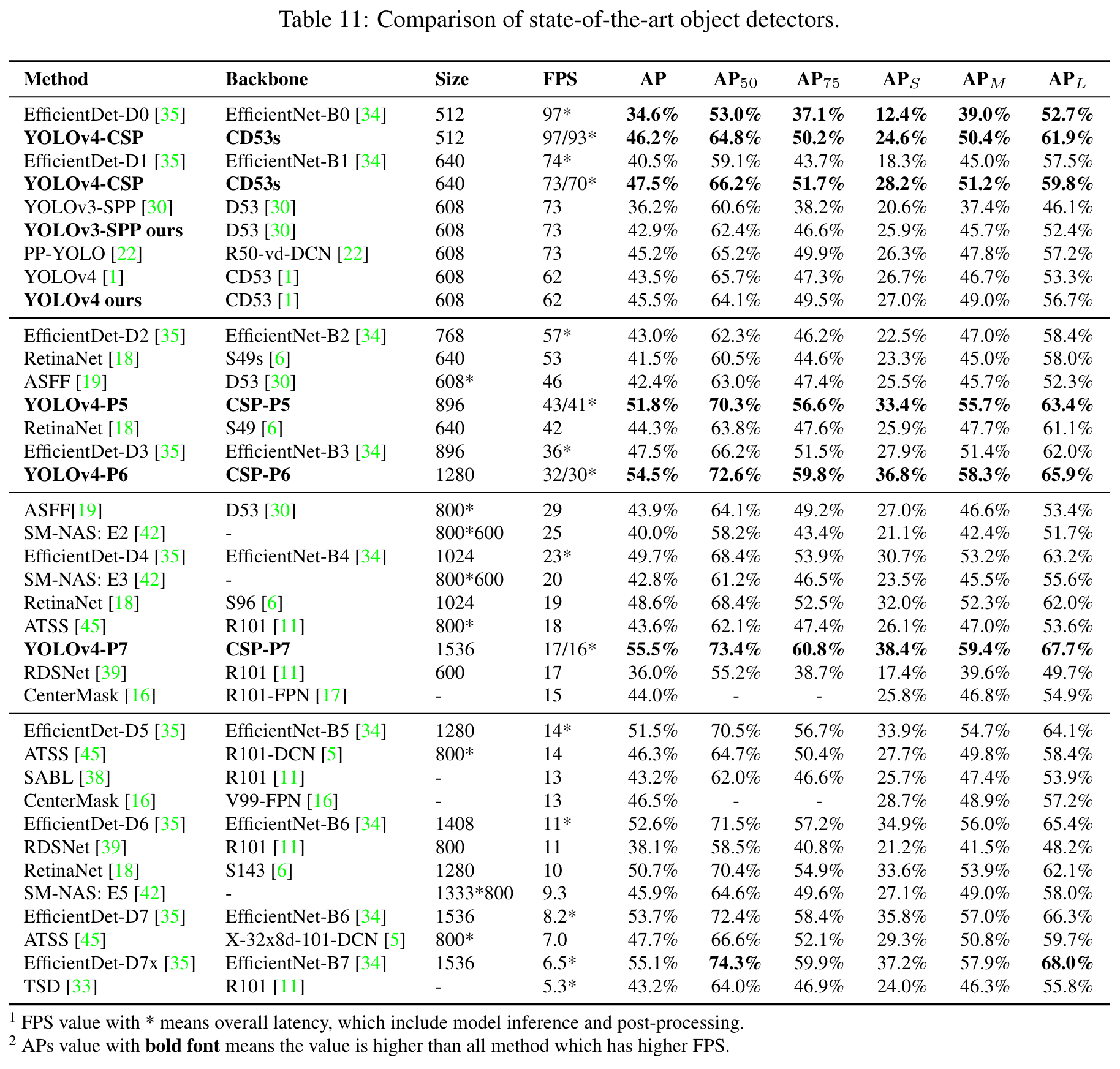
We compare with other real-time object detectors, and the results are shown in Table 11. (Go to Paper)

Highlight

We can see that all scaled YOLOv4 models, including YOLOv4-CSP, YOLOv4-P5, YOLOv4-P6, YOLOv4P7, are Pareto optimal on all indicators. (Go to Paper)

Highlight

When we compare YOLOv4-CSP with the same accuracy of EfficientDetD3 (47.5% vs 47.5%), the inference speed is 1.9 times. (Go to Paper)

Highlight

When YOLOv4-P5 is compared with EfficientDet-D5 with 1303 (Go to Paper)

Highlight

the same accuracy (51.8% vs 51.5%), the inference speed is 2.9 times. (Go to Paper)

Highlight

The situation is similar to the comparisons between YOLOv4-P6 vs EfficientDet-D7 (54.5% vs 53.7%) and YOLOv4-P7 vs EfficientDet-D7x (55.5% vs 55.1%). In both cases, YOLOv4-P6 and YOLOv4-P7 are, respectively, 3.7 times and 2.5 times faster in terms of inference speed. (Go to Paper)

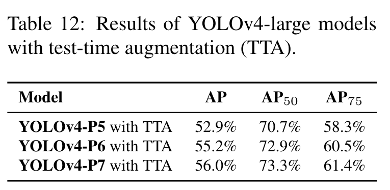
Highlight

The results of test-time augmentation (TTA) experiments of YOLOv4-large models are shown in Table 12. YOLOv4P5, YOLOv4-P6, and YOLOv4-P7 gets 1.1%, 0.7%, and 0.5% higher AP, respectively, after TTA is applied. (Go to Paper)

Image

Image

Highlight

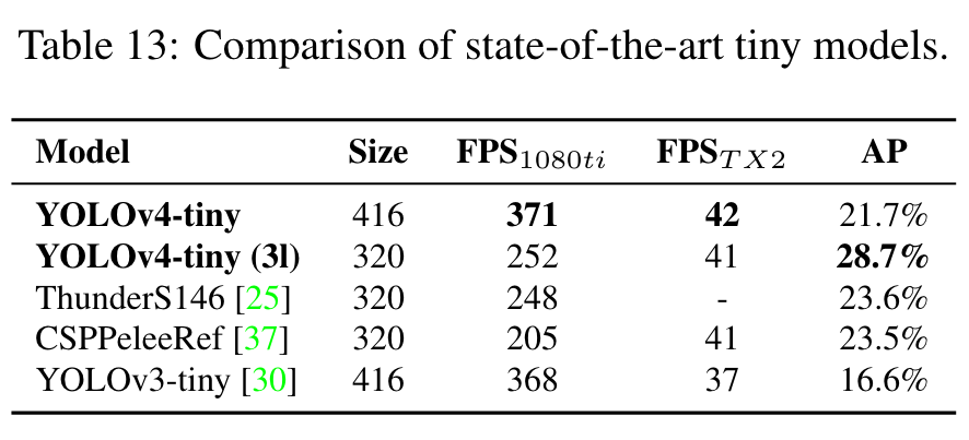
We then compare the performance of YOLOv4-tiny with that of other tiny object detectors, and the results are shown in Table 13. It is apparent that YOLOv4-tiny achieves the best performance in comparison with other tiny models. (Go to Paper)

Image

Image

Highlight

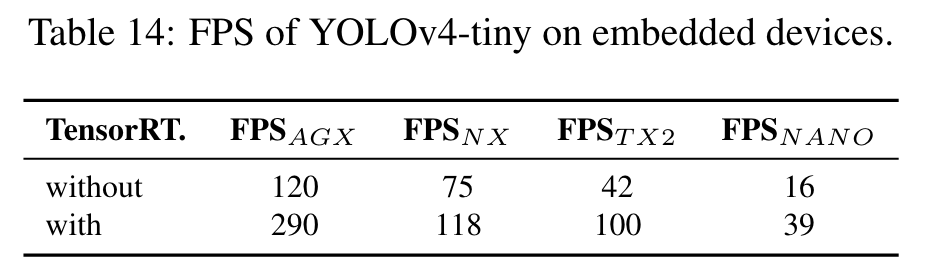
It is apparent that YOLOv4-tiny can achieve real-time performance no matter which device is used. If we adopt FP16 and batch size 4 to test Xavier AGX and Xavier NX, the frame rate can reach 380 FPS and 199 FPS respectively. In addition, if one uses TensorRT FP16 to run YOLOv4-tiny on general GPU RTX 2080ti, when the batch size respectively equals to 1 and 4, the respective frame rate can reach 773 FPS and 1774 FPS, which is extremely fast. (Go to Paper)

Image

Image

5.5. Scaled-YOLOv4 as naı ̈ve once-for-all model

Highlight

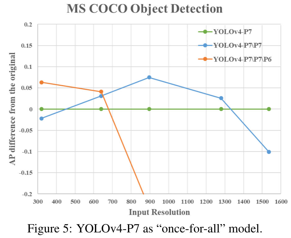
In this sub-section, we design experiments to show that an FPN-like architecture is a na ̈ıve once-for-all model. Here we remove some stages of top-down path and detection branch of YOLOv4-P7. YOLOv4-P7\P7 and YOLOv4P7\P7\P6 represent the model which has removed {P7} and {P7, P6} stages from the trained YOLOv4-P7. Figure 5 shows the AP difference between pruned models and original YOLOv4-P7 with different input resolution. (Go to Paper)

Comment:

이 연구 부분은 FPN과 유사한 아키텍처를 사용한 YOLOv4-P7 모델의 효율성을 탐구합니다. 특히, 모델에서 특정 스테이지를 제거함으로써, 다른 해상도에서의 객체 탐지 성능을 어떻게 최적화할 수 있는지 실험적으로 분석합니다.

Image

Image

Highlight

We can find that YOLOv4-P7 has the best AP at high resolution, while YOLOv4-P7\P7 and YOLOv4-P7\P7\P6 have the best AP at middle and low resolution, respectively. This means that we can use sub-nets of FPN-like models to execute the object detection task well. Moreover, we can perform compound scale-down the model architectures and input size of an object detector to get the best performance (Go to Paper)

Comment:

그 결과, YOLOv4-P7 모델이 높은 해상도에서 가장 우수한 성능을 보였으며, 특정 스테이지를 제거한 모델이 중간 및 낮은 해상도에서 더 좋은 성능을 나타냄을 확인했습니다. 이러한 발견은 객체 탐지 작업을 위한 모델의 아키텍처와 입력 크기를 특정 상황에 맞게 조정할 수 있는 가능성을 시사합니다. 이는 다양한 운영 조건에서 최적의 속도와 정확도의 균형을 달성하는 데 도움이 될 수 있습니다.

6. Conclusions

Highlight

We show that the YOLOv4 object detection neural network based on the CSP approach, scales both up and down and is applicable to small and large networks. (Go to Paper)

Highlight

we achieve the highest accuracy 56.0% AP on test-dev COCO dataset for the model YOLOv4-large, extremely high speed 1774 FPS for the small model YOLOv4-tiny on RTX 2080Ti by using TensorRT-FP16, and optimal speed and accuracy for other YOLOv4 models. (Go to Paper)

---